Cate inference Practice (Causalml-Book)

This is a concise introduction to Chapter 14 of the CausalML(2022) Notebook. (Some of my thoughts are included) For readability, some cells are hidden, but you can run the code by downloading the ipynb file. This practice refers to the paper by Green & Kern (2012). It explores the sentiment of American citizens towards the word “Welfare” using survey data.
The survey subjects are divided into two groups and receive similar but different questions. In particular, it includes questions like “Do you think the government spends too much money on Welfare?” and “Do you think the government spends too much money on Assistance to the Poor?” The survey results show that more people responded affirmatively to the former. (ATE level)
Furthermore, we practice CATE estimation to see how the effect of varying questions differs according to progressive tendencies, education levels, etc.

Setup¶

import numpy as np
import matplotlib.pyplot as plt
from statsmodels.api import OLS
from sklearn.model_selection import StratifiedKFold
from sklearn.model_selection import cross_val_predict
import pandas as pd

# hide

import wget
import os

if os.path.exists('datasets.py'):
    os.remove('datasets.py')
wget.download('https://raw.githubusercontent.com/CausalAIBook/MetricsMLNotebooks/main/T/datasets.py')

if os.path.exists('myxgb.py'):
    os.remove('myxgb.py')
wget.download('https://raw.githubusercontent.com/CausalAIBook/MetricsMLNotebooks/main/T/myxgb.py')

# hide

'myxgb.py'

from datasets import fetch_data_generator

verbose = 0  # Verbosity of auto-ml
n_splits = 5  # Cross-Fitting and Cross-Validation Splits
cfit = True
data = 'welfare'  # Which Dataset, One of {'401K', 'Criteo', 'WELFARE', 'POVERTY', 'Charity'}
plot = True  # wheat to plot result

control_feats = 'all'  # List of Subset of Features to Be Used As Confounders or the String 'All' for Everything
# List of SubSet of Control Features to Be Used for Cate Model or the String 'All' for All Controls
hetero_feats = 'all'
cov_clip = .01  # Clipping of Treatment variance P (x)*(1-p (x))
binary_y = True
random_seed = 1

# Treatment Policy to Evalue
def policy(x):
    return x['polviews'] > 0

# For SEMI-Synthetic Data Generation
semi_synth = False  # Whether True Outcome Y SHOULD Be Replaced by a Fake Outcome from a Known CEF
simple_synth = True  # Whether the True CEF of the Fake Y SHOULD Be Simple or Fitted from Data
max_depth = 2  # max depth of Random Forest During for Semi-Synthetic Model Fitting
scale = .2  # Magnitude of Noise in SEMI-SYNTHETIC DATA


def simple_true_cef(D, X):  # Simple CEF of the Outcome for Semi-Synthetic Data
    return .5 * np.array(X)[:, 1] * D + np.array(X)[:, 1]

get_data, _, _, _ = fetch_data_generator(data=data, semi_synth=semi_synth, simple_synth=simple_synth, scale=scale, true_f=simple_true_cef, max_depth=max_depth)
# hide

# Fetching Dataset
X, D, y, _ = get_data()

Y is the dependent or target variable, D is the variable of interest or treatment variable (whether the wording ‘assistance to the poor’ was used), and X can be thought of as nuisance variables. We only want to know the causal relationship between Y and D, but we have all three because bias would occur if we don’t consider X.

(This is in contrast to prediction models where we only divide into Y (Target Variable) and X (Features).)

D # Here D = 1 means assistance to the poor, D = 0 means welfare wording

array([0, 1, 1, ..., 1, 0, 1])

y # For the statement 'I think the government spends too much money on welfare/assistance to the poor': Yes = 1, No = 0

array([1, 0, 0, ..., 0, 1, 0])

Data Analysis and Simple OLS¶

X.head()

X.describe() # AMONG THESE, PolViews Represents Political Views, with Values from 1 to 7 Becoming more conservative.

X = X - X.mean(axis=0)

plt.figure(figsize=(15, 5))
plt.subplot(1, 2, 1)
plt.hist(D)
plt.title('Treatment')
plt.subplot(1, 2, 2)
plt.hist(y)
plt.title('Outcome')
plt.show()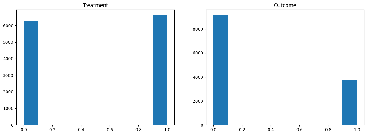

import statsmodels.formula.api as smf

model = smf.ols(formula="y ~ D", data=X).fit(cov_type='HC1')
print(model.summary())

# If not a Random Trial, Selection Bias cannot be excluded by this method.

                            OLS Regression Results                            
==============================================================================
Dep. Variable:                      y   R-squared:                       0.164
Model:                            OLS   Adj. R-squared:                  0.164
Method:                 Least Squares   F-statistic:                     2476.
Date:                Sat, 22 Mar 2025   Prob (F-statistic):               0.00
Time:                        15:33:58   Log-Likelihood:                -6969.7
No. Observations:               12907   AIC:                         1.394e+04
Df Residuals:                   12905   BIC:                         1.396e+04
Df Model:                           1                                         
Covariance Type:                  HC1                                         
==============================================================================
                 coef    std err          z      P>|z|      [0.025      0.975]
------------------------------------------------------------------------------
Intercept      0.4798      0.006     76.111      0.000       0.467       0.492
D             -0.3681      0.007    -49.761      0.000      -0.383      -0.354
==============================================================================
Omnibus:                     1655.598   Durbin-Watson:                   1.990
Prob(Omnibus):                  0.000   Jarque-Bera (JB):             1148.663
Skew:                           0.621   Prob(JB):                    3.72e-250
Kurtosis:                       2.230   Cond. No.                         2.65
==============================================================================

Notes:
[1] Standard Errors are heteroscedasticity robust (HC1)

Doubles-Robust Ate Estimation and CATE Estimation¶

Define and Estimate¶

Before definition of Doubles-Robust Estimator, we will define some functions and estimates. We can create a model that predicts y with all variables (x and d = 0) inside the Control Group with d = 0. Like D = 1, you can create a model. If the two groups are comparable, this may be a good model. (Of course, in some Learners, there may be a chance of being undertected even though it is a policy that creates a predictive value by relying only on X, without considering the effect of 0 or 1 due to the level of covariates.)

\begin{align} g_0 (x): = E [Y \mid D = 0, X = x] \\ g_1 (x): = E [Y \mid D = 1, X = x] \\ g_{D_i} (x): = g_1 (x) * D + g_0 (x) * (1 - D) \\ \end{align}

(1)

You can also make the propensity score model P (x) as follows. Q (x) is a model that predicts Y without using D variable. (It is used for the elementalization method used in DML or CAUSAL FOREST.)

\begin{align} p(x): = E [D \mid X = x] = \ Pr (D = 1 \mid X = x) \\ q(x): = E [Y \mid X = x] \\ \end{align}

(2)

To get all the estimates described here, you can use the desired machine learning. However, when using this method due to over-fitting problems, one rule is to do Cross-Validation. This notebook usually uses xgboost regression.

Now you can estimate the ATE by creating a $Y_i^{DR}$ function as shown below and finding the expected value. The reason why it is called Double Robust is that even if the $\hat{p}(x_i)$ is inaccurate, even if $\hat{g}_1(x_i)$ and $\hat{g}_0(x_i)$ are inaccurate, if the propensity scores estimate $\hat{p}(x_i)$ , the same value is the right ATE.

The Doubly Robust Estimator is defined as follows:

\begin{align} Y_i^{DR}(\hat{g},\hat{p}) := \hat{g}_1(X_i) - \hat{g}_0(X_i) + (Y_i - \hat{g}_{D_i}(X_i))\frac{D_i - \hat{p}(X_i)}{\hat{p}(X_i) (1-\hat{p}(X_i))} \end{align}

(3)

After that, it can be used as follows:

\begin{align} ATE = E_n\left[Y^{DR}(\hat{g},\hat{p})\right], CATE = \tau(X) = E[Y^{DR}(\hat{g}, \hat{p})|X] \end{align}

(4)

Please refer to link for proof.

# Using a function created by the author. XGBOOST does not provide 0/1 binary classification, so wrapper is made separately.

from myxgb import xgb_reg, xgb_clf, RegWrapper

def auto_reg():
    return xgb_reg(random_seed)

def auto_clf():
    return RegWrapper(xgb_clf(random_seed))

modely = auto_clf if binary_y else auto_reg

if cfit:
    cv = StratifiedKFold(n_splits=n_splits, shuffle=True, random_state=random_seed)
    stratification_label = 2 * D + y if binary_y else D
    splits = list(cv.split(X, stratification_label))
else:
    splits = [(np.arange(X.shape[0]), np.arange(X.shape[0]))]

n = X.shape[0]
reg_preds_t = np.zeros(n)
reg_zero_preds_t = np.zeros(n)
reg_one_preds_t = np.zeros(n)

for train, test in splits:
    reg_zero = modely().fit(X.iloc[train][D[train] == 0], y[train][D[train] == 0]) 
    reg_one = modely().fit(X.iloc[train][D[train] == 1], y[train][D[train] == 1]) 
    
    reg_zero_preds_t[test] = reg_zero.predict(X.iloc[test]) # (Y ~ x | d == 0), xgboost
    reg_one_preds_t[test] = reg_one.predict(X.iloc[test]) # (Y ~ x | d == 1), xgBoost
    reg_preds_t[test] = reg_zero_preds_t[test] * (1 - D[test]) + reg_one_preds_t[test] * D[test] # COMBINE Above Two

res_preds = cross_val_predict(modely(), X, y, cv=splits) # (Y ~ x) with CV, xgboost
prop_preds = cross_val_predict(auto_clf(), X, D, cv=splits) # (D ~ x) with CV, XGBOOST

def r2score(y, ypred):
    return 1 - np.mean((y - ypred)**2) / np.var(y)

print(f"R^2 of model for (y ~ X): {r2score(y, res_preds):.4f}")
print(f"R^2 of model for (D ~ X): {r2score(D, prop_preds):.4f}")
print(f"R^2 of model for (y ~ X | D==0): {r2score(y[D==0], reg_zero_preds_t[D==0]):.4f}")
print(f"R^2 of model for (y ~ X | D==1): {r2score(y[D==1], reg_one_preds_t[D==1]):.4f}")
print(f"R^2 of model for (y ~ X, D): {r2score(y, reg_preds_t):.4f}")

R^2 of model for (y ~ X): 0.0458
R^2 of model for (D ~ X): -0.0002
R^2 of model for (y ~ X | D==0): 0.0690
R^2 of model for (y ~ X | D==1): 0.0375
R^2 of model for (y ~ X, D): 0.2140

ATE¶

dr_preds = reg_one_preds_t - reg_zero_preds_t
dr_preds += (y - reg_preds_t) * (D - prop_preds) / np.clip(prop_preds * (1 - prop_preds), cov_clip, np.inf)

ate = np.mean(dr_preds)
print(f"ATE: {ate:.4f}")

ATE: -0.3660

CATE¶

(1) Just estimate¶

If we turn the $Y^{DR}$ as a dependent variable, we can get the CATE. The explanation of the output results of the output results estimates how much ATE is increasing if the X1 increases, for example. If the CATE is larger, it can be interpreted as the effect of the policy as the variable increases. If it’s RCT, you’ll get a value that’s almost the same as the second coefficient from y ~ D + D * x1.

dfX = X.copy()
dfX['const'] = 1
lr = OLS(dr_preds, dfX).fit(cov_type='HC1')
cov = lr.get_robustcov_results(cov_type='HC1')
print(lr.summary())

                            OLS Regression Results                            
==============================================================================
Dep. Variable:                      y   R-squared:                       0.015
Model:                            OLS   Adj. R-squared:                  0.012
Method:                 Least Squares   F-statistic:                     5.090
Date:                Sat, 22 Mar 2025   Prob (F-statistic):           1.29e-24
Time:                        15:34:00   Log-Likelihood:                -15618.
No. Observations:               12907   AIC:                         3.132e+04
Df Residuals:                   12864   BIC:                         3.164e+04
Df Model:                          42                                         
Covariance Type:                  HC1                                         
================================================================================
                   coef    std err          z      P>|z|      [0.025      0.975]
--------------------------------------------------------------------------------
hrs1            -0.0018      0.001     -2.679      0.007      -0.003      -0.000
income          -0.0110      0.006     -1.965      0.049      -0.022   -3.01e-05
rincome         -0.0047      0.004     -1.256      0.209      -0.012       0.003
age              0.0005      0.001      0.600      0.549      -0.001       0.002
polviews        -0.0217      0.006     -3.630      0.000      -0.033      -0.010
educ             0.0003      0.006      0.051      0.959      -0.011       0.011
earnrs           0.0067      0.012      0.546      0.585      -0.017       0.031
sibs             0.0021      0.003      0.766      0.444      -0.003       0.007
childs           0.0050      0.007      0.724      0.469      -0.008       0.018
occ80        -5.333e-05   4.21e-05     -1.266      0.205      -0.000    2.92e-05
prestg80        -0.0011      0.001     -1.521      0.128      -0.003       0.000
indus80       6.473e-05   3.02e-05      2.145      0.032    5.58e-06       0.000
res16            0.0009      0.005      0.176      0.861      -0.009       0.010
reg16           -0.0024      0.003     -0.813      0.416      -0.008       0.003
family16         0.0076      0.004      1.714      0.087      -0.001       0.016
parborn          0.0028      0.005      0.571      0.568      -0.007       0.013
maeduc           0.0062      0.003      2.407      0.016       0.001       0.011
degree           0.0312      0.013      2.391      0.017       0.006       0.057
hompop          -0.1143      0.061     -1.879      0.060      -0.234       0.005
babies           0.1233      0.062      1.993      0.046       0.002       0.245
preteen          0.1086      0.061      1.766      0.077      -0.012       0.229
teens            0.1383      0.062      2.238      0.025       0.017       0.260
adults           0.1261      0.062      2.034      0.042       0.005       0.248
partyid_1.0     -0.0054      0.024     -0.229      0.819      -0.052       0.041
partyid_2.0      0.0256      0.027      0.944      0.345      -0.028       0.079
partyid_3.0     -0.0239      0.028     -0.868      0.386      -0.078       0.030
partyid_4.0     -0.0808      0.031     -2.583      0.010      -0.142      -0.019
partyid_5.0     -0.0664      0.027     -2.435      0.015      -0.120      -0.013
partyid_6.0     -0.0906      0.033     -2.749      0.006      -0.155      -0.026
partyid_7.0      0.0403      0.069      0.588      0.557      -0.094       0.175
wrkstat_2.0      0.0069      0.026      0.261      0.794      -0.045       0.058
wrkslf_2.0       0.0166      0.023      0.732      0.464      -0.028       0.061
marital_2.0      0.0417      0.046      0.903      0.366      -0.049       0.132
marital_3.0      0.0354      0.023      1.540      0.124      -0.010       0.080
marital_4.0      0.0470      0.042      1.118      0.263      -0.035       0.129
marital_5.0      0.0517      0.022      2.308      0.021       0.008       0.096
race_2           0.0160      0.023      0.690      0.490      -0.030       0.062
race_3           0.0355      0.033      1.086      0.278      -0.029       0.100
mobile16_2.0    -0.0033      0.018     -0.179      0.858      -0.039       0.033
mobile16_3.0     0.0206      0.018      1.137      0.256      -0.015       0.056
sex_2           -0.0662      0.016     -4.124      0.000      -0.098      -0.035
born_2.0        -0.0113      0.042     -0.270      0.787      -0.093       0.071
const           -0.3660      0.007    -51.157      0.000      -0.380      -0.352
==============================================================================
Omnibus:                      833.669   Durbin-Watson:                   1.990
Prob(Omnibus):                  0.000   Jarque-Bera (JB):              605.788
Skew:                           0.430   Prob(JB):                    2.85e-132
Kurtosis:                       2.377   Cond. No.                     6.04e+03
==============================================================================

Notes:
[1] Standard Errors are heteroscedasticity robust (HC1)
[2] The condition number is large, 6.04e+03. This might indicate that there are
strong multicollinearity or other numerical problems.

# Get the CATE of the Income with OLS and see if it is similar.

df_cate_by_ols = X.copy()
df_cate_by_ols['y'] = y
df_cate_by_ols['D'] = D
df_cate_by_ols['D_income'] = D * df_cate_by_ols["income"]
model = smf.ols(formula="y ~ D + income + D_income", data=df_cate_by_ols).fit(cov_type='HC1')
print(model.summary())

                            OLS Regression Results                            
==============================================================================
Dep. Variable:                      y   R-squared:                       0.169
Model:                            OLS   Adj. R-squared:                  0.169
Method:                 Least Squares   F-statistic:                     857.8
Date:                Sat, 22 Mar 2025   Prob (F-statistic):               0.00
Time:                        15:34:00   Log-Likelihood:                -6933.5
No. Observations:               12907   AIC:                         1.388e+04
Df Residuals:                   12903   BIC:                         1.390e+04
Df Model:                           3                                         
Covariance Type:                  HC1                                         
==============================================================================
                 coef    std err          z      P>|z|      [0.025      0.975]
------------------------------------------------------------------------------
Intercept      0.4795      0.006     76.345      0.000       0.467       0.492
D             -0.3677      0.007    -49.843      0.000      -0.382      -0.353
income         0.0265      0.004      7.055      0.000       0.019       0.034
D_income      -0.0188      0.004     -4.419      0.000      -0.027      -0.010
==============================================================================
Omnibus:                     1524.518   Durbin-Watson:                   1.993
Prob(Omnibus):                  0.000   Jarque-Bera (JB):             1119.140
Skew:                           0.619   Prob(JB):                    9.59e-244
Kurtosis:                       2.261   Cond. No.                         4.37
==============================================================================

Notes:
[1] Standard Errors are heteroscedasticity robust (HC1)

Cate for Income. The OLS coefficient and value of the Income for DOUBLY ROBUST Y estimates are almost the same as expected.

(2) Estimating CATE with Confidence Interval¶

Below is to look at the CATE with Confidence Interval based on Joint Inference.

V = cov.cov_params()
S = np.diag(np.diagonal(V)**(-1 / 2))
epsilon = np.random.multivariate_normal(np.zeros(V.shape[0]), S @ V @ S, size=(1000))
critical = np.percentile(np.max(np.abs(epsilon), axis=1), 95)
stderr = np.diagonal(V)**(1 / 2)
lb = cov.params - critical * stderr
ub = cov.params + critical * stderr
jointsummary = pd.DataFrame({'coef': cov.params,
                             'std err': stderr,
                             'lb': lb,
                             'ub': ub,
                             'statsig': ['' if ((l <= 0) & (0 <= u)) else '**' for (l, u) in zip(lb, ub)]},
                            index=dfX.columns)
jointsummary

grid = np.unique(np.percentile(dfX['polviews'], np.arange(0, 110, 20)))

Zpd = pd.DataFrame(np.tile(np.median(dfX, axis=0, keepdims=True), (len(grid), 1)),
                   columns=dfX.columns)
Zpd['polviews'] = grid

pred_df = lr.get_prediction(Zpd).summary_frame()
preds, lb, ub = pred_df['mean'].values, pred_df['mean_ci_lower'].values, pred_df['mean_ci_upper'].values
preds = preds.flatten()
lb = lb.flatten()
ub = ub.flatten()
plt.errorbar(Zpd['polviews'], preds, yerr=(preds - lb, ub - preds))
plt.xlabel('polviews')
plt.ylabel('Predicted CATE (at median value of other features)')
plt.show()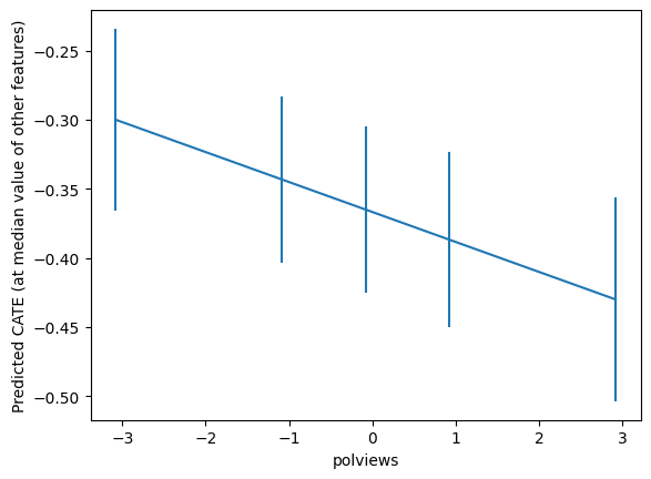

Simpler Best Linear Projections of Cate¶

These are also possible.

There are seven different values of PolViews, and each value can see CATE and Confidence Interval.
If PolViews is a continuous variable, I think we can see how the CATE will change.

from statsmodels.formula.api import ols
df = X.copy()
df['dr'] = dr_preds
lr = ols('dr ~ C(polviews)', df).fit(cov_type='HC1')

grid = np.unique(np.percentile(X['polviews'], np.arange(0, 102, 2)))
Xpd = pd.DataFrame(np.tile(np.median(X, axis=0, keepdims=True), (len(grid), 1)),
                   columns=X.columns)
Xpd['polviews'] = grid
pred_df = lr.get_prediction(Xpd).summary_frame(alpha=.1)

plt.plot(Xpd['polviews'], pred_df['mean'])
plt.fill_between(Xpd['polviews'], pred_df['mean_ci_lower'], pred_df['mean_ci_upper'], alpha=.4)
plt.xlabel('polviews' + ' (other features fixed at median value)')
plt.title('Predicted CATE BLP: cate ~ C(polviews)')
plt.ylabel('CATE')
plt.show()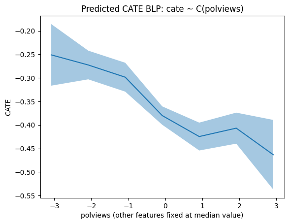

from statsmodels.formula.api import ols
df = X.copy()
df['dr'] = dr_preds
lr = ols('dr ~ polviews', df).fit(cov_type='HC1')

grid = np.unique(np.percentile(X['polviews'], np.arange(0, 102, 2)))
Xpd = pd.DataFrame(np.tile(np.median(X, axis=0, keepdims=True), (len(grid), 1)),
                   columns=X.columns)
Xpd['polviews'] = grid
pred_df2 = lr.get_prediction(Xpd).summary_frame(alpha=.1)

plt.plot(Xpd['polviews'], pred_df2['mean'])
plt.fill_between(Xpd['polviews'], pred_df2['mean_ci_lower'], pred_df2['mean_ci_upper'], alpha=.4)
plt.xlabel('polviews' + ' (other features fixed at median value)')
plt.ylabel('CATE')
plt.title('cate ~ polviews' )
plt.show()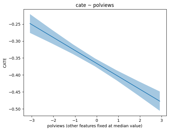

Non-parametric confidence intervals on cate predictions¶

Let’s not like a linear model, but now let’s predict nonparametric CATE. Usually uses access called Causal Forests or Doubly Robust Forests.

Causal Forests¶

Z = X

min_samples_leaf = 50
max_samples = .4

from econml.grf import CausalForest

yres = y - res_preds # Res_PREDS: (y ~ x) with CV, xgboost
Dres = D - prop_preds # Prop_PREDS: (D ~ X) with CV, XGBOOST
cf = CausalForest(4000, criterion='het', max_depth=None,
                  max_samples=.4,
                  min_samples_leaf=50,
                  min_weight_fraction_leaf=.0,
                  random_state=random_seed)
cf.fit(Z, Dres, yres)

top_feat = np.argsort(cf.feature_importances_)[-1]
print(Z.columns[top_feat])

polviews

grid = np.unique(np.percentile(Z.iloc[:, top_feat], np.arange(0, 105, 5)))
Zpd = pd.DataFrame(np.tile(np.median(Z, axis=0, keepdims=True), (len(grid), 1)),
                   columns=Z.columns)
Zpd.iloc[:, top_feat] = grid

preds, lb, ub = cf.predict(Zpd, interval=True, alpha=.1)
preds = preds.flatten()
lb = lb.flatten()
ub = ub.flatten()
plt.errorbar(Zpd.iloc[:, top_feat], preds, yerr=(preds - lb, ub - preds))
plt.xlabel(Zpd.columns[top_feat])
plt.ylabel('Predicted CATE (at median value of other features)')
plt.show()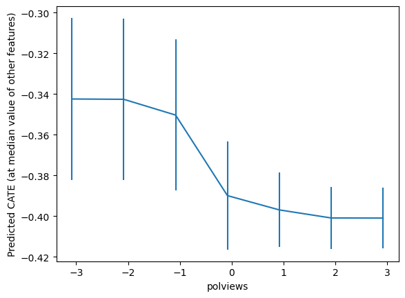

important_feats = Z.columns[np.argsort(cf.feature_importances_)[::-1]]
important_feats[:4]

Index(['polviews', 'indus80', 'educ', 'hrs1'], dtype='object')

plt.figure(figsize=(10, 7))
for it, feature in enumerate(important_feats[:4]):
    plt.subplot(2, 2, it + 1)
    grid = np.unique(np.percentile(Z[feature], np.arange(0, 105, 5)))
    Zpd = pd.DataFrame(np.tile(np.median(Z, axis=0, keepdims=True), (len(grid), 1)),
                       columns=Z.columns)
    Zpd[feature] = grid

    preds, lb, ub = cf.predict(Zpd, interval=True, alpha=.1)
    preds = preds.flatten()
    lb = lb.flatten()
    ub = ub.flatten()
    plt.errorbar(Zpd[feature], preds, yerr=(preds - lb, ub - preds))
    plt.xlabel(feature)
    plt.ylabel('Predicted CATE')
plt.tight_layout()
plt.show()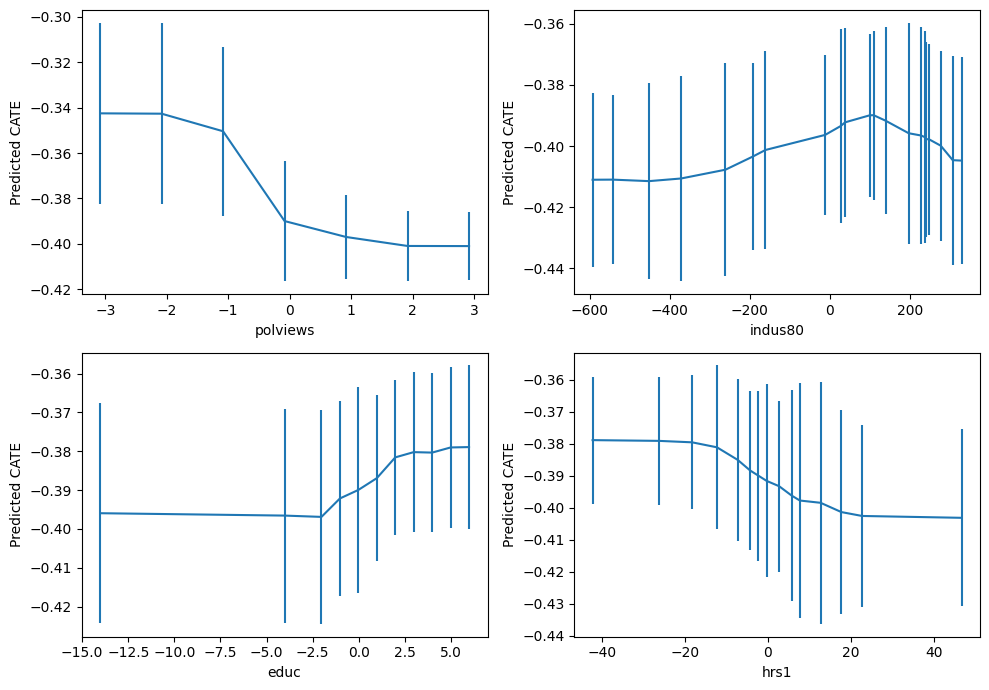

Double Robust Forests¶

from econml.grf import RegressionForest

drrf = RegressionForest(4000, max_depth=5,
                        max_samples=.4,
                        min_samples_leaf=50,
                        min_weight_fraction_leaf=.0,
                        random_state=random_seed)
drrf.fit(Z, dr_preds)

top_feat = np.argsort(drrf.feature_importances_)[-1]
print(Z.columns[top_feat])

polviews

grid = np.unique(np.percentile(Z.iloc[:, top_feat], np.arange(0, 105, 5)))
Zpd = pd.DataFrame(np.tile(np.median(Z.values, axis=0, keepdims=True), (len(grid), 1)),
                   columns=Z.columns)
Zpd.iloc[:, top_feat] = grid

preds, lb, ub = drrf.predict(Zpd, interval=True, alpha=.1)
preds = preds.flatten()
lb = lb.flatten()
ub = ub.flatten()
plt.errorbar(Zpd.iloc[:, top_feat], preds, yerr=(preds - lb, ub - preds))
plt.xlabel(Zpd.columns[top_feat])
plt.ylabel('Predicted CATE (at median value of other features)')
plt.show()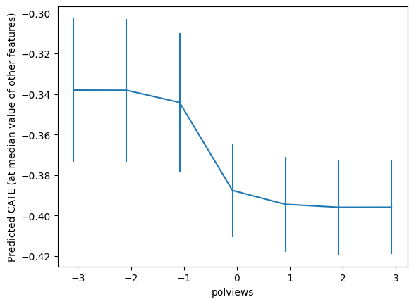

important_feats = Z.columns[np.argsort(drrf.feature_importances_)[::-1]]
important_feats[:4]

Index(['polviews', 'indus80', 'educ', 'hrs1'], dtype='object')

plt.figure(figsize=(10, 7))
for it, feature in enumerate(important_feats[:4]):
    plt.subplot(2, 2, it + 1)
    grid = np.unique(np.percentile(Z[feature], np.arange(0, 105, 5)))
    Zpd = pd.DataFrame(np.tile(np.median(Z, axis=0, keepdims=True), (len(grid), 1)),
                       columns=Z.columns)
    Zpd[feature] = grid

    preds, lb, ub = drrf.predict(Zpd, interval=True, alpha=.1)
    preds = preds.flatten()
    lb = lb.flatten()
    ub = ub.flatten()
    plt.errorbar(Zpd[feature], preds, yerr=(preds - lb, ub - preds))
    plt.xlabel(feature)
    plt.ylabel('Predicted CATE')
plt.tight_layout()
plt.show()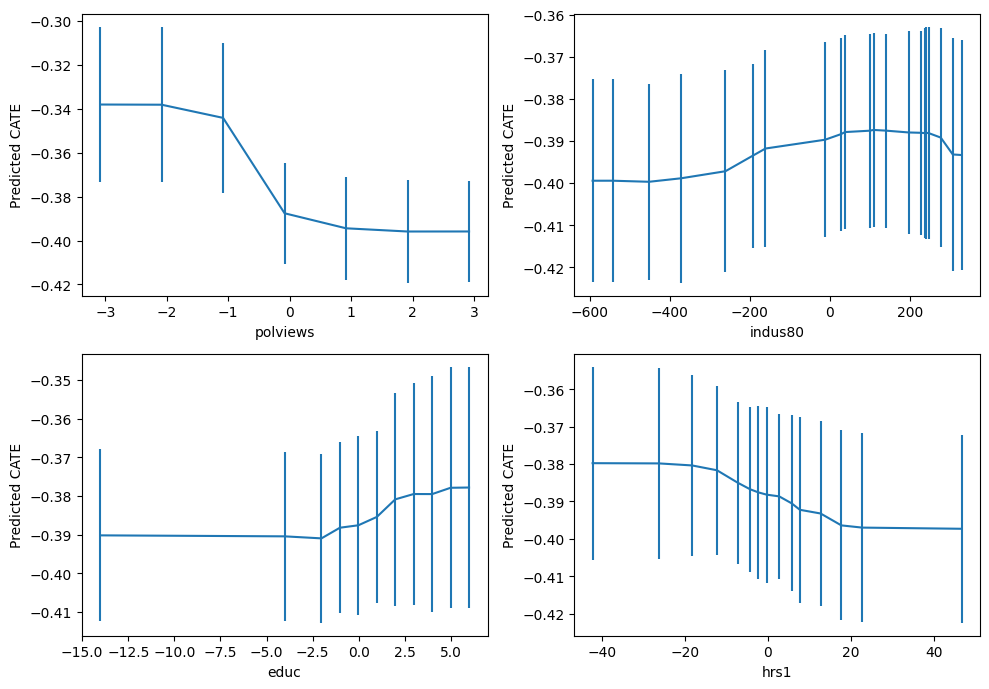

Policy Evaluation¶

Let’s assume that efforts to change words are expensive to reduce the negative perception of the word ‘welfare’. The utility value of Treatment Cost and policy creates a trade-offs relationship. In this case, we will simply put the Treatment Cost in the same unit as the Treatment Effect and make it easier to compare. If it is much more expensive than the ATE -0.36, it will be good to trade only to some of the CATE, and if the cost is not high, it may be better to perform uniform treatment to everyone.

def policy(x):
    return x['polviews'] > 0

Low Cost¶

# Treating by Personized Policy When Cost is Low

treatment_cost = -.3

pi = (dr_preds - treatment_cost) * policy(Z)
score_personalized_low = np.mean(pi)
stderr = np.sqrt(np.var(pi) / pi.shape[0])
print(f"Benefit: {score_personalized_low:.5f}, Standard Error: {stderr:.5f}, 95% CI: {score_personalized_low - 1.96 * stderr:.5f}, {score_personalized_low + 1.96 * stderr:.5f}")

Benefit: -0.04181, Standard Error: 0.00449, 95% CI: -0.05061, -0.03301

# Treating Everyone When Cost is Low

treatment_cost = -.3

pi = (dr_preds - treatment_cost)
score_everyone_low = np.mean(pi)
stderr = np.sqrt(np.var(pi) / pi.shape[0])
print(f"Benefit: {score_everyone_low:.5f}, Standard Error: {stderr:.5f}, 95% CI: {score_everyone_low - 1.96 * stderr:.5f} ~ {score_everyone_low + 1.96 * stderr:.5f}")

Benefit: -0.06601, Standard Error: 0.00720, 95% CI: -0.08012 ~ -0.05191

print("If this cost is low,")
if score_personalized_low < score_everyone_low:
    print("Personalized Treatment is a better policy.")
else:
    print("Treating Everyone is a Better Policy.")

If this cost is low,
Treating Everyone is a Better Policy.

High Cost¶

# Treating by Personized Policy When Cost is High

treatment_cost = -.4

pi = (dr_preds - treatment_cost) * policy(Z)
score_personalized_high = np.mean(pi)
stderr = np.sqrt(np.var(pi) / pi.shape[0])
print(f"Benefit: {score_personalized_high:.5f}, Standard Error: {stderr:.5f}, 95% CI: {score_personalized_high - 1.96 * stderr:.5f} ~ {score_personalized_high + 1.96 * stderr:.5f}")

Benefit: -0.00706, Standard Error: 0.00446, 95% CI: -0.01580 ~ 0.00169

# Treating Everyone When Cost is High

treatment_cost = -.4

pi = (dr_preds - treatment_cost)
score_everyone_high = np.mean(pi)
stderr = np.sqrt(np.var(pi) / pi.shape[0])
print(f"Benefit: {score_everyone_high:.5f}, Standard Error: {stderr:.5f}, 95% CI: {score_everyone_high - 1.96 * stderr:.5f} ~ {score_everyone_high + 1.96 * stderr:.5f}")

Benefit: 0.03399, Standard Error: 0.00720, 95% CI: 0.01988 ~ 0.04809

print("In case where the cost is high,")
if score_personalized_high < score_everyone_high:
    print("Personalized Treatment is a Better Policy.")
else:
    print("Treating Everyone is a Better Policy.")

In case where the cost is high,
Personalized Treatment is a Better Policy.

References¶

Green, D. P., & Kern, H. L. (2012). Modeling Heterogeneous Treatment Effects in Survey Experiments with Bayesian Additive Regression Trees. Public Opinion Quarterly, 76(3), 491–511. 10.1093/poq/nfs036

Causal Inference

Doubly Robust Estimator

Causal Inference

Minimum Wage Example Notebook with DiD